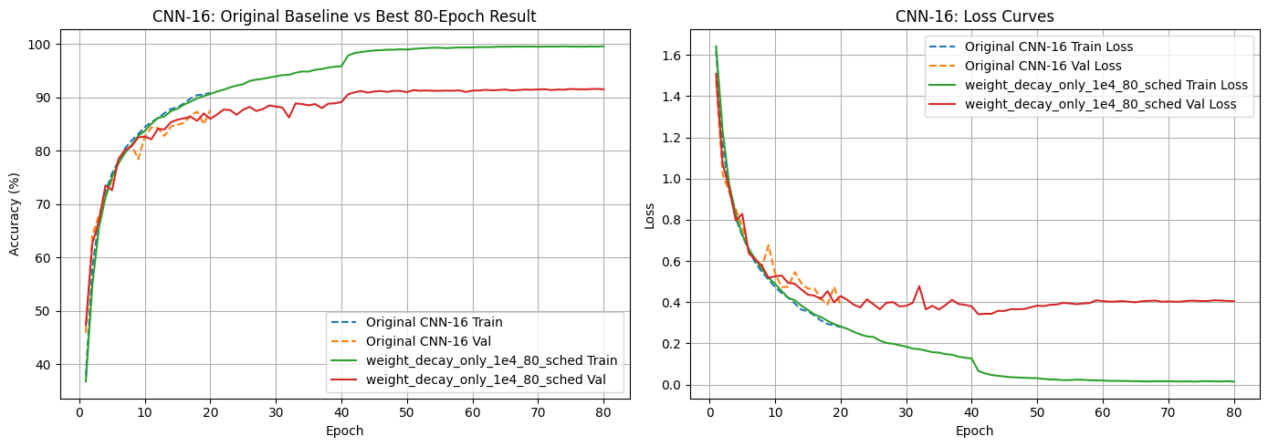
Test accuracy at the checkpoint chosen by validation accuracy, using the 16-layer CNN with weight decay and an 80-epoch training schedule.
What I was trying to find out
Does adding convolutional layers consistently improve image classification? And if an architecture has potential, how much of its performance depends on regularisation, learning-rate scheduling and training duration?
I implemented a linear softmax baseline and configurable convolutional networks in PyTorch, trained multiple variants on CIFAR-10, and compared their behaviour using training, validation and test measurements.
Coursework experiment, not a production model or a published research result. The reported metrics are from the supplied executed notebook.
Keep the comparisons meaningful
CIFAR-10 contains 60,000 colour images across 10 classes. I kept the official test split separate from the train/validation split and used a fixed random seed for repeatable data partitioning. Training images were randomly cropped and flipped, while validation and test images were only normalised.
The notebook defines reusable training and evaluation functions, tracks losses and accuracies across epochs, and uses cross-entropy loss and SGD with momentum. The configurable CNN uses convolution, batch normalisation, ReLU and pooling blocks with a classifier head.
- Dataset
- CIFAR-10 · 32 × 32 RGB · 10 classes
- Framework
- Python · PyTorch · torchvision
- Evaluation
- Train / validation / test accuracy and loss
- Models
- Softmax baseline; 2, 8, 16 and 32-layer CNNs
32 layers performed worse than 8
Moving from 2 to 8 convolutional layers improved test accuracy considerably. Adding layers up to 16 maintained similar performance. But the 32-layer model finished with low training accuracy as well as low validation accuracy. That suggests this run had difficulty optimising the much deeper network—not simply overfitting the training data.
| CNN depth | Validation | Test | Epoch time |
|---|---|---|---|
| 2 layers | 75.68% | 75.42% | 20.9 s |
| 8 layers | 87.64% | 87.43% | 22.7 s |
| 16 layers | 87.63% | 87.83% | 30.8 s |
| 32 layers | 37.21% | 37.15% | 60.3 s |
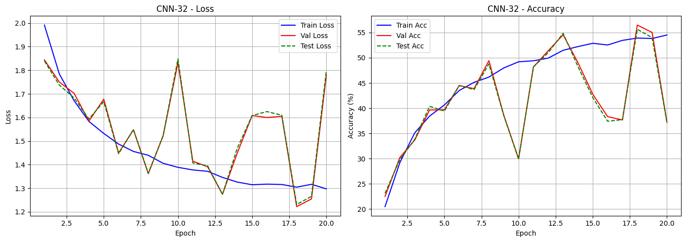
For the improvement phase, I chose CNN-16: the assignment required a 16- or 32-layer deep model, and CNN-16 was considerably more workable.
Training control mattered more than a clever architecture change
The original CNN-16 achieved 87.83% test accuracy. Under a stronger 80-epoch schedule with learning-rate reductions and validation-based checkpoint selection, even the repeated baseline improved. I then compared dropout, weight decay and both together.
| Experiment | Best val. | Test at best val. |
|---|---|---|
| Original 20-epoch baseline | 87.63% | 87.83% |
| 80-epoch baseline, scheduled | 91.38% | 90.77% |
| Dropout only | 91.15% | 91.36% |
| Weight decay (1e-4) | 91.58% | 91.35% |
| Dropout + weight decay | 91.56% | 91.41% |
I selected the weight-decay-only model because it had the highest validation accuracy (91.58%), rather than choosing based on test performance. The combined variant had a slightly higher test score (91.41%), but its validation score was marginally lower. That distinction is worth preserving.
The right setting depended on the training budget
Learning-rate experiments ranged from 0.000001 to 1.0. Under the separate 20-epoch comparison, 0.01 gave the highest test accuracy (86.97%). The 1.0 run collapsed to around chance-level accuracy (10%) while very small rates converged slowly.
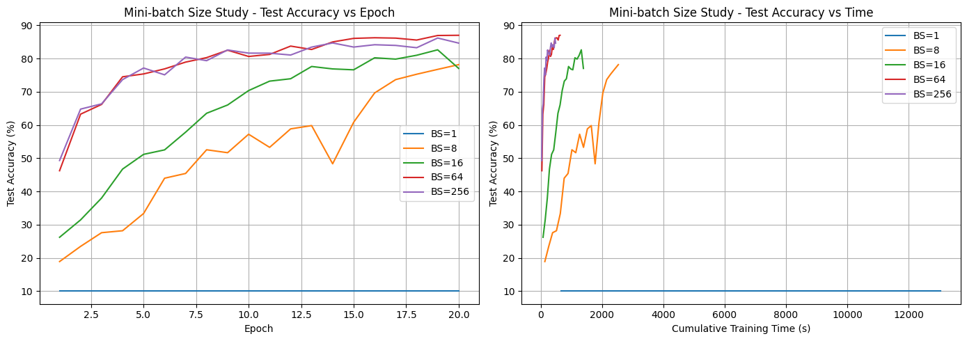
For mini-batches, size 64 reached 87.01% final test accuracy in the 20-epoch study. Size 256 trained faster per epoch but finished at 84.66%. The batch-size-1 run performed at chance level and was particularly slow.
How the experiments were organised
The notebook uses a parameterised CNN class and separate training helpers, so the depth, regularisation and hyperparameter experiments share the same basic process instead of duplicating all model and evaluation code.
- Prepare CIFAR-10 with a seeded train/validation split.
- Define a softmax baseline and reusable CNN architecture.
- Train and log per-epoch loss, accuracy and runtime.
- Compare architectural depth, then improve the selected deep model.
- Select a checkpoint using validation performance and interpret trade-offs.
This is useful experience in writing experiment pipelines and reading model behaviour, rather than simply loading a pre-trained classifier.
What I would change in a more rigorous follow-up
The source notebook logs test-set performance at every epoch. Although the improved checkpoint was selected using validation accuracy, a stricter research pipeline would reserve the test set for a single final evaluation. I would also run multiple random seeds, report variation between runs and consider skip connections for much deeper CNNs.
These results describe particular training configurations, not a universal claim that 32-layer networks are inferior to smaller architectures.
Read the underlying analysis
The figures above were extracted from the executed course notebook, not reconstructed as decorative charts. A shorter, student-ID-free research summary is available as a PDF, with the original source notebook and full submission held back pending a publishing review.
↧Download the portfolio research summaryPDF · selected methods, figures, results and limitationsThe original assignment includes identifying details and assessment material, so it is not automatically distributed as part of this public-facing draft.